ROB 201 Calculus for the Modern Engineer
Where fundamental calculus concepts become algorithms in motion
ROB 201 is a 4-credit, principle-driven path through the calculus engineers actually use: approximation, understanding the whole from simple parts, local linearity, rate-total duality, and differential equations for motion and feedback control.
Thinking about taking ROB 201?
Start with the three questions most students ask.
Will it count toward my degree?
For Robotics majors it is designed as a modern path through the MATH 115, 116, and 216 core. Some pathways need a petition, and Robotics Student Services can help students navigate that process.
How hard is it?
The pace is brisk: plan on about 8 hours a week outside lecture. Help is built in, and asking early is encouraged.
What will I actually build?
Three real projects: reconstructing drone motion, optimizing a platform diver, and stabilizing the BallBot.
Why ROB 201 exists
Many engineering students arrive excited about math, physics, computing, and building things, only to meet a calculus sequence that can feel disconnected from engineering practice.
ROB 201 puts calculus back in contact with the work engineers actually do: modeling robots, integrating sensor data, optimizing motion, solving differential equations, and designing feedback controllers. The course replaces a bag-of-tricks view of calculus with a smaller set of durable ideas.
Students return again and again to approximation, understanding the whole from simple parts, local linearity, rate-total duality, and motion. That repetition is what makes it possible to responsibly connect material traditionally spread across Calculus I, Calculus II, and Ordinary Differential Equations.
For students: what you will learn and build in code
ROB 201 is for students who want calculus to feel useful while they are learning it. The course still teaches core mathematical ideas, but it emphasizes concepts, computation, and applications over long stretches of manual symbolic manipulation.
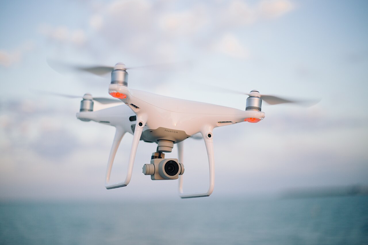
Numerical integration of drone data
Use numerical integration to reconstruct motion from real 3D data, including the practical problem of acceleration drift.
Image: Josh Sorenson, CC0, via Wikimedia Commons.
Constrained optimization
Use gradient descent with equality constraints to model a 10-meter platform diver's motion and prepare for ODE thinking.
Images: licensed Adobe Stock image; ROB 201 course-generated 10-meter platform animation and mechanical model.

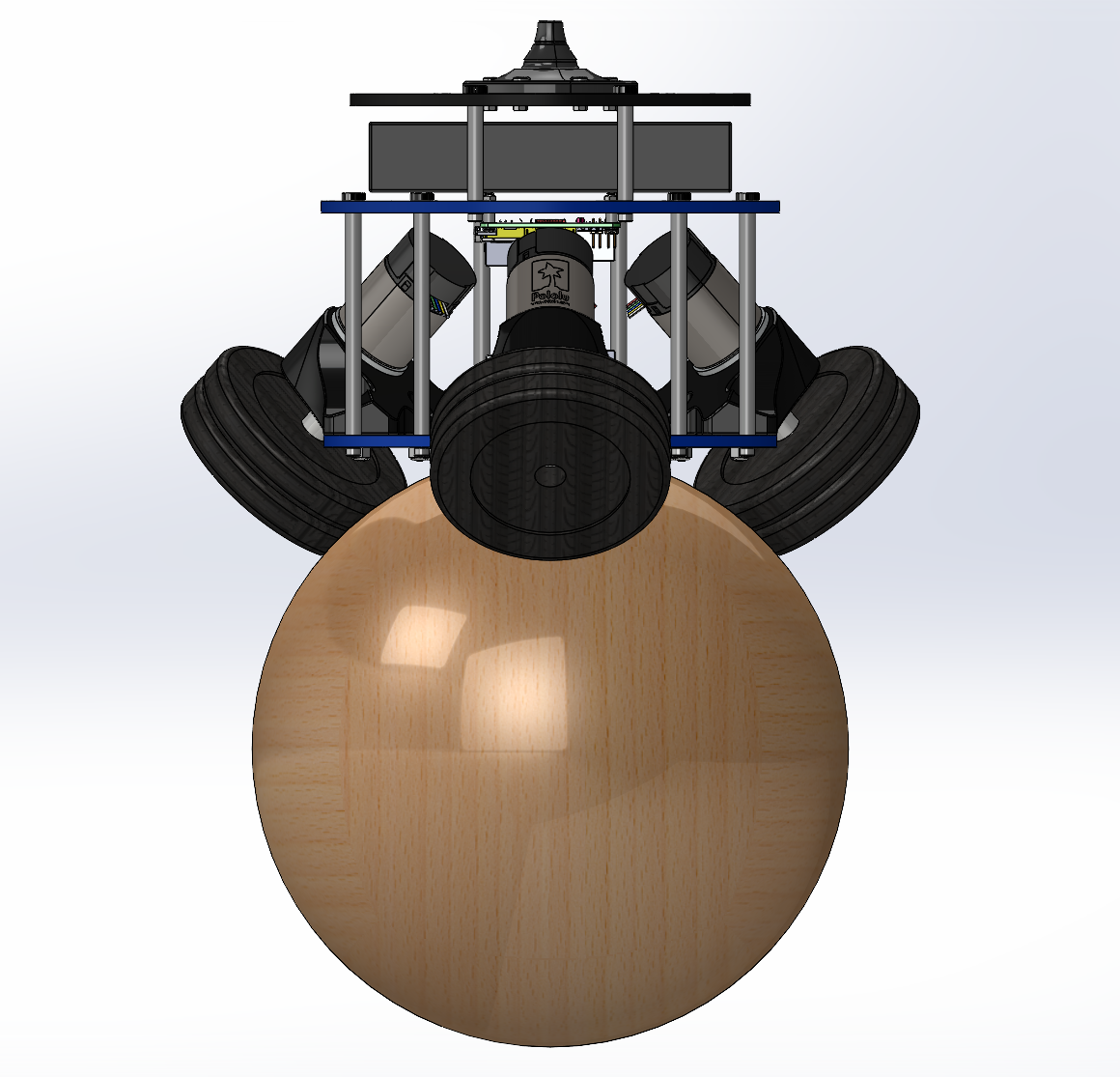
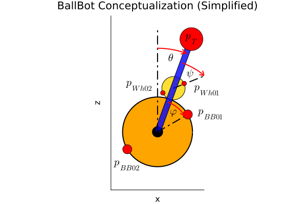
BallBot feedback control
Use ODEs, Laplace transforms, linearization, and feedback control to model and stabilize the ROB 311 BallBot.
Images: ROB 201 course materials.
Is ROB 201 a good fit?
The pace is brisk. Students are most likely to thrive when they can spend about 8 hours per week outside lecture, keep up with weekly work, ask for help early, and enjoy seeing fundamental principles brought to life through applications and computation.
How it counts
For Robotics majors, ROB 201 is designed as a modern path through the core material of MATH 115, MATH 116, and MATH 216. For AY 2025-26, some pathways require a petition, and Robotics Student Services can help students navigate that process. Non-Robotics majors or double majors should consult their own advisors.
The organizing ideas
The course becomes manageable because students keep recognizing the same mathematical moves in new settings.
Approximation
If a quantity cannot be computed directly, trap it between quantities you can compute, then tighten the bounds.
Wholes from simple parts
Break a complicated system into pieces you can understand, write a simple formula for one piece, add the pieces, and take the limit.
Local linearity
Zoom in close enough and nonlinear behavior becomes usable through derivatives, Jacobians, Taylor approximations, Newton's method, and gradient descent.
Motion
Differential equations turn local laws into future behavior. They are how calculus becomes simulation, dynamics, robotics, and feedback control.
Read the fuller preface framing
Calculus for the Modern Engineer is organized around a small number of ideas that show up again and again: approximation, understanding the whole from the sum of its simplest parts, local linearity, rate-total duality, and motion. Calculus is not a bag of tricks. It is how engineers take a world that is curved, distributed, nonlinear, and moving, and turn it into something we can compute, predict, optimize, and control.
One reason this course can responsibly compress the essential material from three traditional courses (Calculus I, Calculus II, and Differential Equations) into one course is that we keep returning to these organizing principles. New formulas are not treated as isolated facts to memorize. They are attached to a short list of durable ideas, and those ideas are reinforced in lectures, Julia demos, homework, and engineering examples. When students can see the same principle behind area, center of mass, gradient descent, robot dynamics, and feedback control, the course becomes smaller in the mind even while its applications become larger.
Limits: The Ultimate Get-Out-of-Jail-Free Card
Limits put calculus on a sound foundation. Whenever the math looks shaky, a careful limit is often the move that restores order. Infinity? Take a limit. A function misbehaves? Take one-sided limits. An integral runs off to forever? Take a limit. A formula looks illegal until the last second? Take the limit carefully and see what survives.
Limits are how calculus keeps its promises.
Where this principle is taught and reinforced: Lectures 01 to 02 introduce limits through Archimedes' approximation principle and limits at infinity. Lectures 06 to 08 develop one-sided limits, continuity, and the Squeeze Theorem. Lecture 16 uses limits as the "Get Out of Jail Free Card" for improper integrals. Lectures 21 to 22 return to limits in the setting of Laplace transforms and signals.
Archimedes' Approximation Principle: Trap the Quantity
Archimedes taught us one of the deepest moves in mathematics: if you cannot compute a quantity directly, trap it between quantities you can compute. Build a lower estimate. Build an upper estimate. Tighten both. If the two estimates close in on the same value, the unknown quantity has nowhere left to go.
Today, one version of this idea is called the Squeeze Theorem, or Sandwich Theorem. But the principle is much bigger. It is how calculus defines and computes areas under general curves, volumes, arc lengths, moments of inertia, and other quantities the Greeks could not even dream of.
This is not a trick. This is the essence of calculus.
Where this principle is taught and reinforced: Lecture 01 introduces Archimedes' computation of π by upper and lower polygonal estimates and uses the same idea to begin area under a curve. Lectures 02 to 04 turn this into limits and Riemann lower and upper sums. Lecture 08 gives the modern Squeeze Theorem and shows how upper and lower bounds rescue difficult examples. Lectures 16 to 17 use comparison ideas for improper integrals. Lecture 27 returns to bounding, approximation, and numerical computation in larger engineering problems.
Understanding the Whole from the Sum of Its Simplest Parts: The Amazing Power of the Rectangle
Engineers often understand a small piece of a system long before they understand the entire system. Calculus exploits this fact. Break a complicated object into infinitesimally small pieces, write a simple formula for one piece, and then add the pieces together. As the pieces become vanishingly small, the approximation becomes exact.
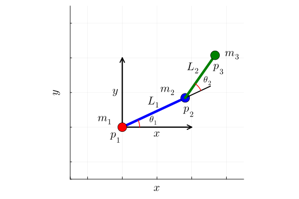
This idea appears throughout engineering. A robot link is not a point mass. It has length, shape, density, center of mass, kinetic energy, potential energy, and moment of inertia. Rather than analyzing the entire link at once, we analyze a tiny piece and then sum the contributions of all the pieces.
The rectangle is the first and most important example of this idea. By slicing a region into thin rectangles and adding their areas, we compute the area under a curve. The same principle later gives us mass from density, center of mass from distributed mass, energy from power, probability from probability density, and moment of inertia from mass distributed throughout an object.
If you truly understand this principle, many intimidating formulas become less mysterious. They are simply different ways of understanding the whole from the sum of its simplest parts.
Where this principle is taught and reinforced: Lecture 01 begins with the "Amazing Power of the Rectangle." Lectures 04 to 05 define and develop the Riemann integral. Lecture 06 applies differentials and integrals to links of a robot with distributed mass. Lectures 12 to 14 use rectangles, disks, washers, shells, path length, energy, and Lagrangian modeling. Lectures 15 to 16 connect accumulated quantities with antiderivatives and improper integrals. Lecture 27 returns to moment of inertia and numerical integration.
Linear Approximation: Make the Nonlinear Usable
The world is nonlinear. Linear algebra is where engineers have power.
Linear approximation is the bridge. Zoom in close enough, and many nonlinear functions behave almost like linear ones. That single idea gives us tangent lines, derivatives, differentials, Taylor approximations, Jacobians, Newton's method, robot linearization, and gradient descent.
Without linear approximation, one of the mathematical engines behind modern optimization and AI would not run.
Where this principle is taught and reinforced: Lecture 09 introduces the derivative and the centrality of local linear approximation. Lectures 10 to 11 develop Taylor approximation, partial derivatives, and Jacobians. Lectures 12 to 13 use derivatives and gradients in optimization and engineering applications. Lectures 19, 25, and 26 use Jacobian linearization to replace nonlinear ODEs and robot equations by linear models that can be analyzed and controlled.
The Fundamental Theorems, or Speedometer-Odometer Duality: Accumulated Rates Build Totals, Differences of Totals Reveal Rates.
Your car knows calculus! What?
Differentiation tells us the instantaneous rate of change. Integration tells us the accumulated total. The Fundamental Theorems of Calculus reveal that these are not separate kingdoms.
Velocity accumulates into position. Acceleration accumulates into velocity. Density accumulates into mass. Power accumulates into energy.
And, under the right conditions, accumulated totals reveal the rates that created them.
This is the hinge of calculus: local change and global accumulation are two sides of the same machine.
Where this principle is taught and reinforced: Lecture 10 previews the idea that differentiation and integration are inverse operations. Lecture 14 prepares the need for integrating robot equations. Lectures 15 to 16 develop antiderivatives and the Fundamental Theorems of Calculus. Lectures 21 to 24 reinforce the same rate-total relationship through Laplace transforms, signals, transfer functions, and linear ODEs.
Differential Equations: Local Laws Create Future Motion
A differential equation is an equation involving a function and its rates of change. Newton's law, F = ma, is a differential equation: force determines acceleration, acceleration changes velocity, and velocity changes position.
This is why differential equations matter to engineers. They let us build models that predict trajectories from local information: physics, chemistry, biology, data, geometry, or control laws.
Differential equations turn local slope information into long-term behavior. They are how calculus becomes simulation, dynamics, robotics, and feedback control.
Where this principle is taught and reinforced: Lectures 13 to 14 derive differential equations from mechanical and energy-based models. Lectures 17 to 20 introduce ODEs, numerical methods, existence and uniqueness, linear systems, matrix exponentials, and linearization. Lectures 21 to 24 use Laplace transforms and transfer functions to solve and analyze linear ODEs. Lectures 25 to 26 connect ODEs to transient response, feedback design, and nonlinear robot models. Lecture 27 reinforces numerical and modeling ideas in larger engineering problems.
Evidence from ROB 101: the precedent matters
ROB 201 is not Michigan Robotics' first computational mathematics course. ROB 101 Computational Linear Algebra was created in 2020 and has now seen more than a thousand students pass through its doors. That experience matters for adoption: it shows that an application-centered, computation-forward math course can prepare students for demanding downstream work.
The ROB 101 evidence summarized here comes from the EEI Days 2026 session "Robotics 101: Assessing a discipline-specific linear algebra course". The assessment was conducted by Michigan Robotics in collaboration with CRLT and CRLT-Engin, including Dr. Heather Rypkema, a founding member of the Foundational Course Initiative team, former Assessment & Analytics specialist, and Head of Learning Analytics and Associate Director of the Foundational Course Initiative at CRLT.
Students reach advanced courses earlier
ROB 101 students reached machine-learning coursework earlier than students who took MATH 214.
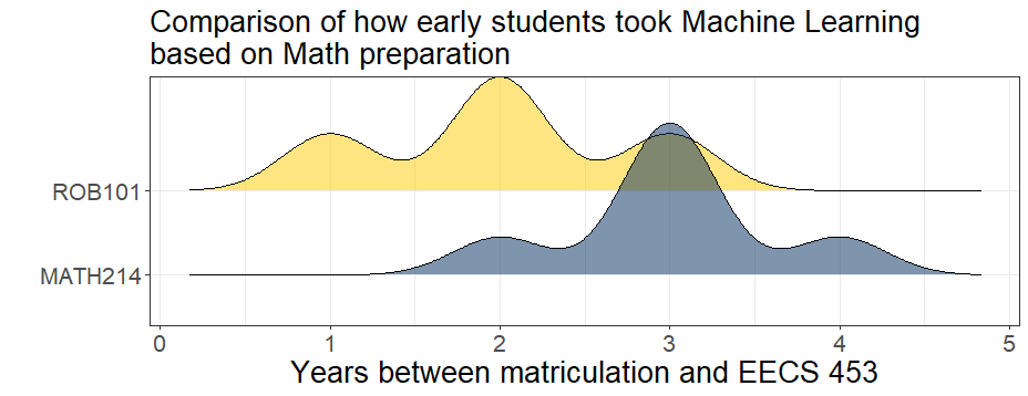
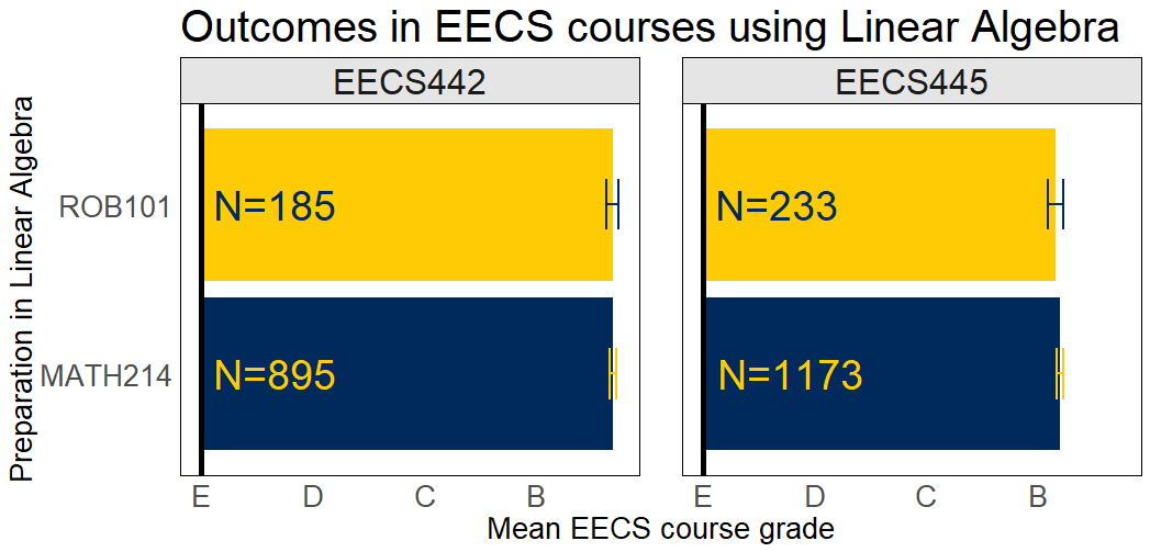
Downstream outcomes are comparable
In EECS 442 Computer Vision and EECS 445 Machine Learning, grade outcomes for ROB 101 and MATH 214 students were not statistically different.
The implication for ROB 201: the question is not whether Michigan Robotics can design serious math courses. ROB 101 has already shown that students can move earlier into advanced technical work and perform comparably once they arrive, with additional ROB 101 assessment findings pointing to more equitable grade outcomes and higher College of Engineering retention rates for students who took the course.
For instructors and potential adopters
ROB 201 was built around three pillars: numerical integration, constrained optimization, and feedback control. These projects give the course a beginning, middle, and end while repeatedly reinforcing the same underlying ideas.
Course design
- Integrates single-variable differential and integral calculus, vector derivatives, ordinary differential equations, and Laplace transforms.
- Uses Julia, Jupyter-style assignments, symbolic tools, numerical methods, and feedback-control examples.
- Begins with summation and numerical integration, separates antiderivative techniques from the idea of integration, and introduces ODE structure before the formal ODE unit.
- Includes proofs and rigor in the textbook for instructors and curious students, while keeping the main student experience application-centered.
What students need clarified
Student feedback in April 2025 indicated uncertainty about whether ROB 201 would satisfy downstream course prerequisites outside Robotics.
IOE has updated their prerequisites. ME 240 is accepting ROB 201 through the petition process for its math prerequisite/co-requisite path. ECE is accepting ROB 201 as a prerequisite for EECS 215 and EECS 216 upon petition. Robotics Student Services will help with the petition process for anyone who asks.
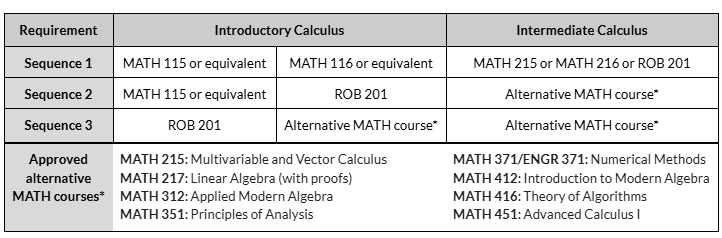
Degree requirements and prerequisites must be separated
Michigan Engineering has a common math core built around MATH 115, MATH 116, and MATH 216. Departments can accept alternate paths through that core for their own degrees, and separately, departments can adjust prerequisites for their own courses.
- IOE
- IOE has updated their prerequisites to recognize the ROB 201 pathway.
- MECHENG 240
- ME 240 is accepting ROB 201 through the petition process for its math prerequisite/co-requisite path.
- ECE / EECS
- ECE is accepting ROB 201 as a prerequisite for EECS 215 and EECS 216 upon petition.
- Student support
- Robotics Student Services will help with the petition process for anyone who asks.
Prof. Kevin Pipe has contacted the instructors of the following courses about treating ROB 201 as equivalent or acceptable for prerequisite purposes.
| Course | Prerequisite treatment |
|---|---|
| AEROSP 201 | MATH 116 or equivalent; accept ROB 201 as equivalent. |
| AEROSP 205 | MATH 116 or ROB 201. |
| AEROSP 215 | MATH 216 or ROB 201. |
| BIOMEDE 211 | MATH 216, 256, 286, or ROB 201. |
| BIOMEDE 231 | MATH 116, 156, 186, 121, or ROB 201. |
| BIOMEDE 517 | MATH 216 or ROB 201. |
| EECS 203 | MATH 115, 116, 119, 120, 121, 156, 175, 176, 185, 186, 214, 215, 216, 217, 255, 256, 285, 286, 295, 296, 417, 419, ROB 101, or ROB 201. |
| EECS 215 | MATH 116, 121, 156, or ROB 201. |
| MECHENG 240 | Co-requisite of MATH 216, 256, 286, or 316; allow ROB 201 as a prerequisite. |
For communications and media
The short story is that ROB 201 turns calculus from a gatekeeper into a gateway. It gives engineering students a one-semester, principle-driven path through the calculus they need for robotics, control, computation, and later math-intensive courses.
Public message
Michigan Robotics is rethinking the undergraduate math sequence by teaching calculus through computation, modeling, and control.
Why it matters
The course helps students see calculus as an engineering tool rather than a barrier course, while preserving rigor and connecting to advanced work.
Adoption angle
ROB 201 builds on the ROB 101 precedent: students can move earlier into advanced technical courses and succeed when they get there.
Resources
Everything you need to evaluate the course or share it, gathered in one place.
Course GitHub
Lecture recordings, lecture notes, homework sets, programming materials, and project overview.
Open repositoryMath pathways
Suggested paths through additional math courses for Robotics students.
Open pathways PDF